Reinventing the 'property clock'

For many years, the ‘property clock’ has been a useful tool for investors to maximise returns through careful analysis of market cycles. 

In 2020, however, the property clock has been found wanting, as the unprecedented economic uncertainty of the coronavirus crisis has made market cycles volatile and future movements difficult to predict.

Property analytics firm Higher than Average Growth (HtAG) has developed a research methodology that addresses the limitations of the property clock, and provides investors with a more nuanced approach that remains useful even during unexpected events.

HtAG’s Growth Rate Cycle (GRC) represents the rate of change in median value year on year and is a little different to the property clock.

The best way to highlight this difference is to explain the philosophy behind the GRC and the property clock cycle notions.

GRC vs the property clock

The property clock is tied to the change of value of a particular property market. As changes in the property values are cyclical, their movements follow a trend that moves from a peak to a bottom and to a peak again. 

Finder.com.au defines the property clock in the following way:

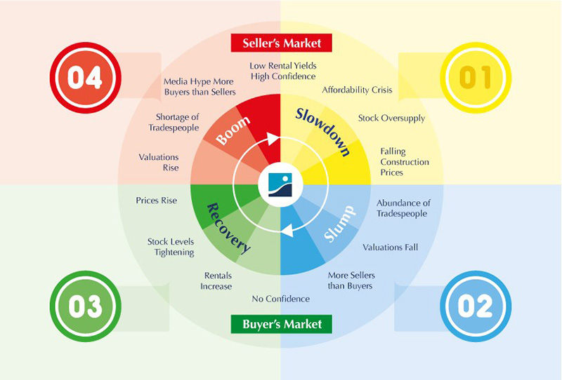
“The property clock is a useful method of tracking the property market cycle. It is based on the recognised stages of the property cycle: a “boom” followed by a downswing in prices, “bust” as the market hits the bottom of the cycle, and then a recovery period as the market builds towards the next boom. 

This clearly-defined cycle can be expressed in the form of a clock. When the hour hand on the clock is at 12, the property market is in a boom period, demand is outpacing supply and prices are at their peak. 

As the hand moves down, clockwise around the face, the market enters a downswing period. Prices start to cool until, when the hand reaches 6, there is an oversupply of houses and the market bottoms out.”

The usefulness of understanding the property clock is that an investor can utilise the cyclical movements of the property market to maximise returns. Finder.com.au goes on to note:

“The property clock makes a nice graphic and is a useful illustration of market performance, but it also serves a practical purpose. By working out where a particular suburb sits on the clock, you can time the market just right to get the best value for money. 

That is, selling at the peak and buying when prices are at their lowest. The property clock offers an extra degree of certainty and reliability when predicting which regions and suburbs are ripe for investment.

It can help new investors gain a better understanding of the property market and the dependable cycle it follows. Once you have a better understanding of the different periods of market performance, you can examine patterns and market trends to establish exactly where a certain region sits on the property clock.”

GRC, on the other hand, is tied to the change in the rate of growth in the median price as opposed to the median dollar value of a property market. Its differences with the property clock have to be nuanced – it represents a much more sensitive way of assessing movements of a particular area.

The property clock depicts price movements within one property cycle that spans from 8-10 years. As such, the property clock would suggest that within those 8-10 years, prices move following a more or less stable pattern, moving from a peak, declining to reach a bottom, rising from the bottom to reach a peak, and so on. 

Given that properties are an illiquid asset, meaning that transactions and subsequent price movements are not as fast and sporadic as that of shares, it benefits the investor to ascertain the property clock of a particular area to time the market right to get the best value for money. 

In simple terms, buying at the peak will result in a diminished return on investment, as any subsequent price movement will be one of loss, while buying at the bottom will result in an increased ROI as prices have nowhere else to go but up.

HtAG’s GRC deals with the inherent weakness and limitation of the property clock, most of which pertains to the preconceived idea that property markets behave in a more or less stable and predictable fashion, meaning that reduction in the median value of a locality after prices have peaked is inevitable and certain. 

As noted by Finder.com.au:

“While the property clock is undoubtedly a useful tool for home buyers and investors, it does have a few key limitations you should be aware of. It’s worth remembering that the property clock is basically used to predict the future, so there’s always a risk of unexpected economic or market developments producing a deviation in the property cycle.”

This means that the property clock is an isolated snapshot which presupposes particular movements of an area irrespective of actual market conditions.

As such, although it suggests markets move cyclically, it nonetheless does not appropriately consider historical price movements to account for what Finder.com.au terms as ‘unexpected’ economic conditions: considering a large enough timescale, one would be able to consider price movements more holistically and adequately accounting for all sudden and not so sudden changes in the property investment landscape.

Busting the myth about declining markets

Busting myth one: declining market equals a decrease in the median value.

The subtle but important difference between macro and micro-movements of an area is that property market ‘movements’ follow two different patterns simultaneously, respective to the time frame and characteristics of interest (price or percentage growth) in question. 

If one focuses on the change in the median value within a time frame of eight to 10 years, it can be said that the movements are somewhat cyclical and predictable in such a way that a peak is followed by a bottom and vice versa. 

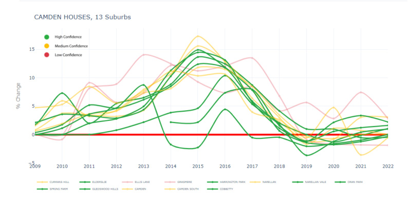
This is evident when looking at the graph below, which highlights that nearly all suburbs combined in Camden Council follow a pattern of bottoming at about 2009, rising to reach a peak at about 2015, then decline to a previous bottom at the 2019-2022 interval.

The macro-scale of the property clock would suggest that a declining market, one that is positioned between a peak and a bottom, is always indicative of negative growth (i.e. a reduction in the median value). 

However, if one considers a shorter time scale within the Growth Rate Cycle of Camden Council he or she would realise (irrespective of how counter-intuitive it might seem) that a ‘declining market’ can correspond to positive growth and an increase in the median values.

This is illustrated in the 2016-2018 section of the Camden Council GRC graph below. 

Considering the downward trajectory of the line within these two years, it becomes evident that Camden Council’s rate of growth is ‘declining’. 

However, its ‘growth rate’ is still in between 2 per cent to 12 per cent (y-axis). At its peak in 2015, Camden Council experienced about 15 per cent growth in its median value. 

In 2016, 2017, 2018 on the other hand, its growth was slowing to 12 per cent, 6 per cent, and 2 per cent, respectively.

This information becomes very pertinent for investors with short investment windows (i.e. renovators, flippers, or developers) as it suggests that even though an area is experiencing a decline in its rate of growth, it can still be growing at a five to 10 per cent rate.

To put it in context, if I outlay a $25,000 deposit for an investment property worth $500,0000 (5% of the property value) and the relevant property market experiences 10 per cent growth (albeit a declining one if compared to historical movement), this would mean that in a two-year time scale ‘declining market’ I would have realised 100 per cent ROI (discounting interest rates and tax).

While the GRC provides macro cyclical information allowing customers to determine both the length and stability of the median value growth cycle within a particular area, it also provides the following:

• A more detailed depiction of the area’s cyclical movements suggesting that an area can move between an increase in the rate of growth and a decrease in the rate of growth within a time scale of two years. The GRC highlights patterns in price changes.
• A more nuanced understanding of the price movements by highlighting cyclical changes in the median price in terms of historical and forecasted growth rate. For example, an area’s median value can be decreasing while its negative growth rate can be slowing, indicating that an area has rebounded and is positioned for an imminent increase in its median value. An excellent example of this would be the 2020 point in the Camden Council GRC, which shows that the rate of growth for the area has bottomed and that although 2021 and 2022 will experience negative growth, the trajectory is one of an incline suggesting that the area is positioned for median price increases post 2021-2022.
• ‘Sneak peek’ into what happens before median prices increase. GRC provides a more intelligent timing and planning tool respective to an investment window. An area can experience increases in median value but show signs of a downward trajectory in the rate of growth, which minimises future capitalisation on investment if the investment window is medium to long term, while allowing for suitable investment returns if our investment window is short term.
• A better area ranking tool permitting for a more nuanced ‘investment grading’ of areas in terms of ROI. Homebuyers and property investors can determine the effects of compounded capital growth on their initial investment between different areas of interest which is not available from the ‘property clock’. This becomes especially pertinent when a potential investment is considered alongside an existing property investment portfolio.

The fact that an area can experience growth in median value at its downturn in the rate of growth, brings me to another significant benefit of using the GRC as an integral element of property investment decision-making. 

It simplifies the assessment of areas in terms of market fundamentals, which usually require the investor to collate and analyse statistics on a plethora of additional variables. The GRC feature minimises the complexity of astute investment decision-making.

GRC and market fundamentals

Busting myth two: supply and demand ratio understanding requires a correlation between multiple variables.

The cycle highlighted on the last chart above becomes specifically meaningful when compared against other areas’ cycles. 

Lengthier cycles would suggest that property values spend longer at peaks and bottoms, which becomes pertinent when considering timing the market to get the best value for money. 

More importantly, lengthier and smooth cycles are indicative of solid market fundamentals. 

Not only does this eliminate the need to inquire into other variables, as it has already been represented in the solid and steady historical movements within the cycle, but it also becomes a useful benchmark when superimposed against areas that exhibit shorter and more sporadic cycles indicative of some ‘one industry’ Councils.

A crucial point – and one which is at the core of HtAG’s GRC – would be: why make the property investment process more complicated than it needs to be by considering a plethora of elements such as household information, demographics, affordability, credit policy, national wealth, wage and job creation, the supply of dwellings and consumer confidence, before making a decision when all of those elements, although beneficial, are already embedded within the historical movement of the rate of growth for an area and its projected rate of growth values?

HtAG’s argument is that one should not need to be an economist or a savvy property investment professional with decades of experience to be able to invest in property. 

In respect to this, I have some food for thought – would an area with unsolid market fundamentals such as weak population growth, high unemployment and oversupply follow the same GRC pattern as one presented for Camden Council? The best way to answer this question is with an illustration.

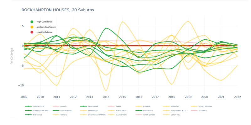
The graph below represents the growth rate cycle of Rockhampton in Queensland. 

2016 Census data suggests Rockhampton’s population was 79,726 people, which was close to Camden’s population of 78,216.

Looking at the GRC for the two Council areas and considering that both areas have a nearly identical population, it is safe to say that Camden has much better market fundamentals than Rockhampton. 

This is a conclusion that can be reached by merely looking at the graph without spending days and weeks collecting, tabulating and analysing statistics on household information, demographics, affordability, credit policy, national wealth, wage and job creation, the supply of dwellings, and consumer confidence for the two respective areas.

The static and isolated nature of the property clock would provide no service because it would not ‘contextualise’ the existing position of an area within a cycle by considering the current cycle position in terms of its historical movements. 

When superimposing Rockhampton and Camden, the property clock would suggest that Camden had reached its bottom. At the same time, Rockhampton could also be classified in the same way, or even highlighted as a rising market. 

However, this information alone would not really depict the investment potential of the two areas.

Although both areas are potentially positioned for growth as a result of being located at the bottom or rising part of the cycle, Rockhampton cycles have not been as steady and clearly defined as Camden’s, while also predominantly sitting in the negative growth section of the graph.

This is where we come to one of the benchmarks HtAG has introduced for assessing an area based on GRC, which eliminates the requirement of employing general economic modelling to determine the effect population and unemployment, for example, have on price movements. 

The Negative Growth Rule suggests that investment potential of an area diminishes respective to the number of times the area has ventured into negative growth territory (growth rate below zero red lines in the Rockhampton graph) as it suggests that the supply and demand relationship is imbalanced in such a way that it minimises the customer’s opportunity for taking advantage of compounded capital growth.

Although Camden Council represents a better investment opportunity than Rockhampton Council, both have experienced negative growth on some occasions which negatively impacted the investment grading of the areas. 

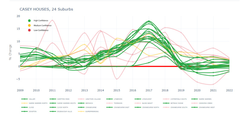
This could mean that Rockhampton has a imbalance in the supply and demand ratio, which is either founded on weak population growth, an oversupply of properties, higher trending unemployment, or a combination of all three, making it an unsuitable investment locality when benchmarked against a locality which shows a stable pattern in its growth rate cycle but has not experienced strong negative growth in the past.  

For example, Casey City on the diagram below.

Even though in the last ten years some property professionals considered Rockhampton as a solid investment locality, there is no need to venture outside of the HtAG platform (and source additional data) to determine why Rockhampton has been hovering around zero growth line for the past 13 years and is more than likely not positioned to rebound to a level that would make it an investment-grade locality any time soon. 

At least not until 2022 as the forecast suggests.

One critical aspect of knowing the ‘historical behaviour of the area’ is to ascertain the number of times the growth rate of the locality has been negative.

In addition to needing to know the ‘stability’ of median value changes, it is also very useful to know if the area has experienced negative growth on more than one occasion.

Areas that continuously fall in the negative-growth category can be described as areas with weak market fundamentals or areas that have an imbalanced relationship between supply and demand.

This realisation was not reached quickly. Our regression analysis suggests that external variables rarely have an impact on price growth within a particular area. 

Determining which variable (i.e. population growth, unemployment, building approvals, etc.) correlates best with price growth is a superfluous process. 

If one variable has a strong influence on price growth in a particular location, this influence, more often than not, cannot be replicated elsewhere.

Every property market is unique and there is no one hard and fast rule that can be applied to model its’ median value trends based on the traditional ‘fundamental variables’. 

Growth and decline cycle is the only stable and unchanging component that applies to all property markets in Australia. 

Because of this, using the GRC as a proxy to market fundamentals, one can ascertain the investment grade of an area by simply comparing its’ compounded capital growth potential to other prospect markets and thus shortlist high ROI markets with ease.